Regions of genome plasticity analyses

Purpose

Regions of Genome Plasticity (RGPs) are clusters of genes made of shell and cloud genomes in the pangenome graph. Most of them arise from Horizontal gene transfer (HGT) and correspond to Genomic Islands (GIs). RGPs from different genomes can be grouped in spots of insertion based on their conserved flanking persistent genes, rather than their gene content, to find out which are located in the same locations in the genome. The panRGP methods and its subcommands and subsequent output files are made to detect describe as thoroughly as possible those Regions of Genome Plasticity across all genomes of the pangenome.

Those methods were supported by the panRGP publication which can be read to have their methodological descriptions and justifications.

PanRGP

This command works exactly like workflow. The difference is that it will run additional analyses to characterize Regions of Genome Plasticity (RGP).

--- title: "Workflow Overview: Steps launched by the panrgp command" align: center --- %%{init: {'theme':'default'}}%% graph LR i[input genomes] --> a r:::panrgp s:::panrgp subgraph Pangenome creation a:::workflow c:::workflow g:::workflow p:::workflow a("annotate") --> c c(cluster) --> g(graph) g(graph) --> p(partition) end subgraph Region of Genomic Plasticity p --> r(rgp) r --> s(spot) end p --> f[pangenome.h5] s --> f[pangenome.h5] classDef panrgp fill:#84d191 classDef panmodule fill:#d44066 classDef workflow fill:#d4ae40

You can use the panrgp with annotation (gff3 or gbff) files with --anno option, as such:

ppanggolin panrgp --anno genomes.gbff.list

For fasta files, you need to use the alternative --fasta option, as such:

ppanggolin panrgp --fasta genomes.fasta.list

Just like workflow, this command will deal with the annotation, clustering, graph and partition commands by itself. Then, the RGP detection is ran using rgp after the pangenome partitioning. Once all RGP have been computed, those found in similar genomic contexts in the genomes are gathered into spots of insertion using spot.

If you want to tune the rgp detection, you can use the rgp command after the workflow command. If you wish to tune the spot detection, you can use the spot command after the rgp command. Additionally, you have the option to utilize a configuration file to customize each detection within the panrgp command.

More detail about RGP detection and the spot of insertion prediction can be found in the panRGP publication

RGP detection

Once partitions have been computed, you can predict the Regions of Genome Plasticity. This subcommand’s options are about tuning parameters for the analysis.

You can do it as such:

ppanggolin rgp -p pangenome.h5

This will predict RGP and store results in the HDF5 file.

This command has 5 options that will directly impact the method’s results. If you are not sure to understand what they do, you should not change their values as they’ll probably behave exactly the way you want them to. The options --variable_gain, --persistent_penalty are both linked to each other. They will impact respectively by how much a persistent gene will penalize the prediction of a RGP, and oppositely how a variable gene (shell, cloud, or multigenic persistent) will promote the prediction of a RGP. The --min_score is the filter that will classify a genome region as RGP or not. Users looking to change those 3 parameters should consider reading the Materials and Methods of the panRGP publication to fully understand how those values impact the prediction.

The two other options are more straightforward. The --min_length will indicate the minimal size in base pair that a RGP should be to be predicted. The --dup_margin is a filter used to identify persistent gene families to consider as multigenic. Gene families that have more than one gene in more than --dup_margin genomes will be classified as multigenic, and as such considered as “variable” genes.

After this command is executed, a single output file that will list all of the predictions can be written, the regions_of_genomic_plasticity.tsv file.

Spot prediction

To study RGP that are found in the same area in different genomes, we gather them into ‘spots of insertion’. These spots are groups of RGP that do not necessarily have the same gene content but have similar bordering persistent genes. We run those analyses to study the dynamic of gene turnover of large regions in bacterial genomes. In this way, spots of the same pangenome can be compared and their dynamic can be established by comparing their different metrics together. Detailed descriptions of these metrics can be found in the RGP and spot output section.

Spots can be computed once RGP have been predicted. You can do that using:

ppanggolin spot -p pangenome.h5

This command has 3 options that can change its results:

--set_size defines the number of the bordering persistent genes that will be compared. (default: 3)
--overlapping_match defines the minimal number of bordering persistent genes that must be identical and in the same order to consider two RGP borders as being similar. This means that, when comparing two borders, if they overlap by this amount of persistent genes they will be considered similar, even if they start or stop with different genes. (default: 2)
--exact_match_size Defines the minimal number of firstly bordering persistent genes to consider two RGP borders as being similar. If two RGP borders start with this amount of identical persistent gene families, they are considered similar. (default: 1)

The two other options are related to the ‘spot graph’ used to predict spots of insertion.

--spot_graph writes the spot graph once predictions are computed
--graph_formats defines the format in which the spot graph is written. Can be either gexf or graphml. (default: gexf)

You can the use the dedicated subcommand draw to draw interactive figures for any given spot with the python library bokeh. Those figures can can be visualized and modified directly in the browser. This plot is described here

Multiple files can then be written describing the predicted spots and their linked RGP, such as a file linking RGPs with their spots and a file showing multiple metrics for each spot.

RGP outputs

RGP

The regions_of_genomic_plasticity.tsv is a tsv file that lists all the detected Regions of Genome Plasticity. This requires to have run the RGP detection analysis by either using the panrgp command or the rgp command.

It can be written with the following command:

ppanggolin write_pangenome -p pangenome.h5 --regions -o rgp_outputs

The file has the following format :

Column	Description
region	A unique identifier for the region. This is usually built from the contig it is on, with a number after it.
genome	The genome it is in. This is the genome name provided by the user.
contig	Name of the contig
genes	The number of genes included in the RGP.
first_gene	Name of the first gene of the region
last_gene	Name of the last gene of the region
start	The start position of the RGP in the contig.
stop	The stop position of the RGP in the contig.
length	The length of the RGP in nucleotide
coordinates	The coordinates of the region. If the region overlap the contig edges will be right with join coordinates syntax (i.e 1523..1758,1..57)
score	Score of the RGP.
contigBorder	This is a boolean column. If the RGP is on a contig border it will be True, otherwise, it will be False. This often can indicate that, if an RGP is on a contig border it is probably not complete.
wholeContig	This is a boolean column. If the RGP is an entire contig, it will be True, and False otherwise. If a RGP is an entire contig it can possibly be a plasmid, a region flanked with repeat sequences or a contaminant.

RGP to gene families

The rgp_families.tsv is a TSV file that maps each RGP to its gene family content.

It can be written with the following command:

ppanggolin write_pangenome -p pangenome.h5 --regions_families -o rgp_outputs

Column	Description
rgp_id	The RGP identifier (found in ‘region’ column of `regions_of_genomic_plasticity.tsv`).
family_id	The gene family identifier present in the RGP.

Spots

The spots.tsv is a tsv file that links the spots in summarize_spots.tsv with the RGPs in regions_of_genomic_plasticity.tsv.

It can be created with the following command:

ppanggolin write_pangenome -p pangenome.h5 --spots -o rgp_outputs

Column	Description
spot_id	The spot identifier (found in the ‘spot’ column of `summarize_spots.tsv`).
rgp_id	The RGP identifier (found in ‘region’ column of `regions_of_genomic_plasticity.tsv`).

Summarize spots

The summarize_spots.tsv file is a tsv file that will associate each spot with multiple metrics that can indicate the dynamic of the spot.

It can be created with the following command:

ppanggolin write_pangenome -p pangenome.h5 --spots -o rgp_outputs

Column	Description
spot	The spot identifier. It is unique in the pangenome.
nb_rgp	The number of RGPs present in the spot.
nb_families	The number of different gene families that are found in the spot.
nb_unique_family_sets	The number of RGPs with different gene family content. If two RGPs are identical, they will be counted only once. The difference between this number and the one provided in ‘nb_rgp’ can be a strong indicator on whether their is a high turnover in gene content in this area or not.
mean_nb_genes	The mean number of genes on RGPs in the spot.
stdev_nb_genes	The standard deviation of the number of genes in the spot.
max_nb_genes	The longest RGP in number of genes of the spot.
min_nb_genes	The shortest RGP in number of genes of the spot.

Borders

Each spot has at least one set of gene families bordering them. To write the list of gene families bordering spots, you can use the --borders option as follow:

ppanggolin write_pangenome -p pangenome.h5 --borders -o rgp_outputs

It will write a .tsv file with 4 columns:

Column	Description
spot_id	The spot identifier. It is unique in the pangenome.
number	The number of RGPs present in the spot that have those bordering genes.
border1	Comma-separated list of gene families of the 1st border.
border2	Comma-separated list of gene families of the 2nd border.

Since there can be some variation in the borders, some spots will have multiple borders and thus multiple lines in this file. The sum of the number for each spot_id should be exactly the number of RGPs in the spot.

In addition, the --borders option also generates a file named border_protein_genes.fasta, containing protein sequences corresponding to the gene families of the spot borders.

Draw spots

The draw command with the option --draw_spots can draw specific spots of interest, whose ID are provided, or all the spots if you wish. It will also write a gexf file, which corresponds to the gene families and their organization within the spots. It is basically a subgraph of the pangenome, consisting of the spot itself. The command can be used as such:

ppanggolin draw -p pangenome.h5 --draw_spots --spots all

This command draws an interactive .html figure and a .gexf graph file for all the spots.

If you are interested in only a single spot, you can use its identifier to draw it. For example for the spot_34:

ppanggolin draw -p pangenome.h5 --draw_spots --spots spot_34

The interactive figures that are drawn look like this:

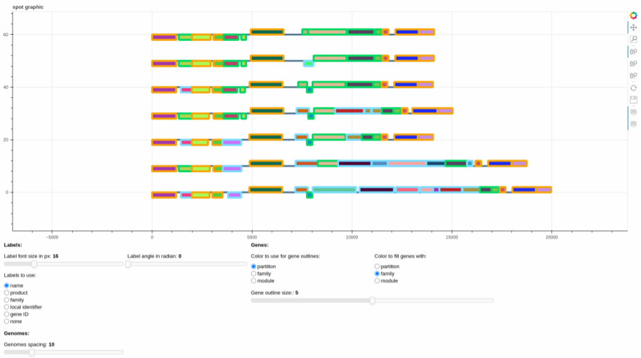
The plot represents the different gene organizations that are found in the spot. If there are RGPs with identical gene organization, the organization is represented only once (the represented RGP is picked at random among all identical RGPs). The list of RGPs with the same organization is accessible in the file written alongside the figure called spot_X_identical_rgps.tsv, with X the spot_id.

They can be edited using the sliders and the radio buttons, to change various graphical parameters, and then the plot itself can be saved using the save button on the right of the screen, if need be.

For the gexf file, you can see how to visualize it in the section about the pangenome gexf.

RGP clustering

To cluster RGP (Regions of Genome Plasticity) based on their gene families, you can use the command panggolin rgp_cluster. The panggolin rgp_cluster command performs the following steps to cluster RGP based on their gene families:

Calculation of GRR (Gene Repertoire Relatedness): The command calculates the GRR values for all pairs of RGP. The GRR metric evaluates the similarity between two RGP by assessing their shared gene families.
Graph Construction: The command constructs a graph representation of the RGP, where each RGP is represented as a node in the graph. The edges between the nodes are weighted using the GRR values, indicating the similarity of the two RGP.
Filtering GRR Values: GRR values below the --grr_cutoff threshold (default 0.8) are filtered out to remove noise from the analysis.
Louvain Communities Clustering: The Louvain communities clustering algorithm is then applied to the graph. This algorithm identifies clusters of RGPs with similar gene families.

There are three modes available for calculating the GRR value: min_grr, max_grr, or incomplete_aware_grr.

min_grr mode: This mode computes the number of gene families shared between two RGPs and divides it by the smaller number of gene families among the two RGPs.
max_grr mode: In this mode, the number of gene families shared between two RGPs is calculated and divided by the larger number of gene families among the two RGPs.
incomplete_aware_grr (default) mode: If at least one RGP is considered incomplete, which typically happens when it is located at the border of a contig, the min_grr mode is used. Otherwise, the max_grr mode is applied. This mode is useful to correctly cluster incomplete RGP.

The resulting RGP clusters are stored in a tsv file with the following columns:

column	description
RGP	The unique region identifier.
cluster	The cluster id of the RGP.
spot_id	The spot ID of the RGP.

The command also generates the RGP graph in the gexf format, which can be utilized to explore the RGP clusters along with their spots of insertion. In this graph identical RGP with the same family content and with the same spot are merged into a single node to simplify the graph representation. This feature can be disable with the parameter --no_identical_rgp_merging.