Pangenome analyses

Workflow

PPanGGOLiN was created with the idea to make it both easy to use for beginners, and fully customizable for experts. Ease of use has been achieved by incorporating a workflow command that allows the construction and partitioning of a pangenome using genomic data. The command has only one mandatory option, and predefined parameters adapted to pangenomes at the scale of a bacterial species. This command launches the annotation, clustering, graph and partition commands described below.

--- title: "Workflow Overview: Steps launched by the workflow command" align: center --- %%{init: {'theme':'default'}}%% graph LR i[input genomes] --> a subgraph Pangenome creation a:::workflow c:::workflow g:::workflow p:::workflow a("annotate") --> c c(cluster) --> g(graph) g(graph) --> p(partition) end p --> f[pangenome.h5] classDef panrgp fill:#4066d4 classDef panmodule fill:#d44066 classDef workflow fill:#d4ae40

To use this command, you need to provide a tab-separated list of either annotation files (gff3 or gbff) or fasta files. The expected format is detailed in the annotation section

You can use the workflow with annotation files as such:

ppanggolin workflow --anno genomes.gbff.list

For fasta files, you have to change for:

ppanggolin workflow --fasta genomes.fasta.list

Moreover, as detailed in the section about providing your gene families, if you wish to use different gene clustering methods than those provided by PPanGGOLiN, it is also possible to provide your own clustering results with the workflow command as such:

ppanggolin workflow --anno genomes.gbff.list --clusters clusters.tsv

All the workflow parameters are obtained from the commands explained below, except for the --no_flat_files option, which solely pertains to it. This option prevents the automatic generation of the output files listed and described in the pangenome output section. If you are unfamiliar with the output available in PPanGGOLiN, we recommend that you do not use this option, so that all results are automatically generated, even though this may take some time.

Tip

In the workflow CLI, it is not possible to tune all the options available in all the steps. For a fully optimized analysis, you can either launch the subcommands one by one as described below, or you can use the configuration file as described here

Annotation

Annotate from fasta files

As an input file, you can provide a list of .fasta files. If you do so, the provided genomes will be annotated using the following tools:

• Pyrodigal, which is based on Prodigal, to annotate CDSs

• ARAGORN to annotate tRNAs

• Infernal coupled with HMM of the bacterial and archaeal rRNAs downloaded from RFAM to annotate rRNAs.

To proceed with this stage of the pipeline, you need to create an genomes.fasta.list file. This file should be tab-separated with each line depicting an individual genome and its pertinent information with the following organization (only the first two columns are mandatory):

• The first column contains a unique genome name

• The second column contains the path to the associated FASTA file

• The following columns contain Contig identifiers present in the associated FASTA file that should be analyzed as being circular. For the ‘circular contig identifiers,’ if you do not have access to this information, you can safely ignore this part as it does not have a big impact on the resulting pangenome.

You can check this example input file.

To run the annotation part, you can use this minimal command:

ppanggolin annotate --fasta genomes.fasta.list

Use a different genetic code in my annotation step

To annotate the genomes, you can easily change the translation table (or genetic code) used by Pyrodigal just by giving the corresponding number as described here.

Force the Prodigal procedure

Prodigal can predict gene in single/normal mode that includes a training step on your genomes or in meta/anonymous mode, which uses pre-calculated training files. As recommended in the Prodigal documentation: “Anonymous mode should be used on metagenomic data sets, or on sequences too short to provide good training data.”

By default, PPanGGOLiN will determine the best mode based on the contig length. The procedure can be overridden with the option -p, --prodigal_procedure. The option only accepts single or meta keywords, corresponding to the Prodigal procedure name.

Customize the RNA annotation

If you do not want to predict the RNA (and thus not use Infernal and Aragorn), you can add the --norna option to your command. Otherwise, by default, any CDS overlapping RNA genes will be deleted as they are often false positive calls. You can prevent this filtering by using the --allow_overlap option.

Additionally, the --kingdom archaea option can be utilized when working with archaea genomes to specify Infernal’s RNA annotation model.

Use annotation files for your pangenome

You can provide annotation files in either gff3 files or .gbk/.gbff files, or a mix of them. They should be provided through as a list in a tab-separated file that follows the same format as described for the fasta files. You can check this example input file.

Note

Use your own annotation for your genome is highly recommended, particularly if you already have functional annotations, as they can be added to the pangenome.

You can provide them using the following command:

ppanggolin annotate --anno genomes.gbff.list

How to deal with annotation files without sequences

If your annotation files do not contain the genome sequence, you can use both options simultaneously to obtain the gene annotations and gene sequences, as follows:

ppanggolin annotate --anno genomes.gbff.list --fasta genomes.fasta.list

Take the pseudogenes into account for pangenome analyses

By default, PPanGGOLiN will not take pseudogenes into account. However, they could be worth keeping in certain contexts. It is possible to include pseudogenes in the pangenome by using the --use_pseudooption.

Compute pangenome gene families

Cluster genes into gene families

After annotating genomes, their genes will be compared to determine similarities and build gene families using this information.

If .fasta files or annotation files containing gene sequences were provided, clustering can be executed by using the generated .h5 file, as such:

ppanggolin cluster -p pangenome.h5

How to customize MMSeqs2 clustering

Warning

Not all MMSeqs2 options are available in PPanGGOLiN. For a comprehensive overview of MMSeqs2 options, please refer to their documentation. To provide your own custom clustering from MMSeqs2 or another tool, please follow the instructions detailed in the dedicated section.

PPanGGOLiN will run MMseqs2 to perform clustering on all the protein sequences by searching for connected components for the clustering step.

How to set the identity and coverage parameters

PPanGGOLiN enables the setting of two essential parameters for gene clustering: identity and coverage. These parameters can be easily adjusted using --identity (default: 0.8) and --coverage (default: 0.8). The default values were selected as they are empirically effective parameters for aligning and clustering sequences at the species level.

Be aware that if you decrease identity and/or coverage, more genes will be clustered together in the same family. This will ultimately decrease the number of families and affect all subsequent steps.

Note

The chosen coverage mode in PPanGGOLiN requires both protein sequences to be covered by at least the proportion specified by –coverage, though this is modified afterwards by the defragmentation step.

How to set the clustering mode

MMSeqs provides 3 different clustering modes. By default, the clustering mode used is the single linkage (or connected component) algorithm.

Another option is the set cover algorithm, which can be employed using --mode 1.

Additionally, the clustering algorithms of MMseqs, similar to CD-Hit, can be selected with --mode 2 or its low-memory version through --mode 3.

Providing your gene families

It’s possible to provide your own clusters (or gene families); you must have provided the annotations in the first step. For gff3 files, the expected gene identifier is the ‘ID’ field in the 9^th column. In the case of gbff or gbk files, use ‘locus_tag’ as a gene identifier unless you are working with files from MaGe/MicroScope or SEED, where the id in the ‘db_xref’ field is used instead.

You can give your clustering result in TSV file with a single gene identifier per line. This file consist of 2 to 4 columns in function of the information you want to give. See next part to have more information about expected format.

You can do this from the command line:

ppanggolin cluster -p pangenome.h5 --clusters clusters.tsv

If one of the gene in the pangenome is missing in your clustering, PPanGGOLiN will raise an error. To assert the gene into its own cluster (singleton) you can use the --infer_singleton option as such:

ppanggolin cluster -p pangenome.h5 --clusters clusters.tsv --infer_singleton

Note

When you provide your clustering, PPanGGOLiN will translate the representative gene sequence of each family and write it in the HDF5 file.

Assume the representative gene

The minimum information required is the gene family name (first column) and the constituent gene of the family (second column). In that case, PPanGGOLiN will consider that the first line of a cluster (first occurrence of a family name) is also the line with the representative gene indicated.

Here is a minimal example of your clustering file:

Family_A    Gene_1
Family_A    Gene_2
Family_A    Gene_3
Family_B    Gene_4
Family_B    Gene_5
Family_C    Gene_6

--- title: "Pangenome gene families when assuming representative gene" align: center --- %%{init: {'theme':'default'}}%% flowchart TD subgraph C direction TB C6[6] style C6 fill:#00758f end style C rx:150,ry:150 subgraph B direction TB B4[4] B5[5] style B4 fill:#00758f end style B rx:150,ry:150 subgraph A direction TB A1[1] A2[2] A3[3] style A1 fill:#00758f end style A rx:150,ry:150

Specify the representative gene

It’s possible to indicate which gene is the representative gene by adding a third column.

Here is a minimal example of your clustering file with the third column being the representative gene:

Family_A    Gene_1  Gene_2
Family_A    Gene_2  Gene_2
Family_A    Gene_3  Gene_2
Family_B    Gene_4  Gene_4
Family_B    Gene_5  Gene_4
Family_C    Gene_6  Gene_6

--- title: "Pangenome gene families when specifying representative gene" align: center --- %%{init: {'theme':'default'}}%% flowchart TD subgraph C direction TB C6[6] style C6 fill:#00758f end style C rx:150,ry:150 subgraph B direction TB B4[4] B5[5] style B5 fill:#00758f end style B rx:150,ry:150 subgraph A direction TB A1[1] A2[2] A3[3] style A2 fill:#00758f end style A rx:150,ry:150

Indicate fragmented gene

You can indicate if a gene is fragmented by adding a new column. Fragmented genes are marked with an ‘F’ in this final column.

The position of this column depends on whether you include a representative gene column:

• Without a representative gene column, the fragmented gene column should be in the third position.

• With a representative gene column, it should appear in the fourth position.

Example 1: Clustering file without representative gene column (fragmented gene in 3rd column):

Family_A	Gene_1
Family_A	Gene_2
Family_A	Gene_3	F
Family_B	Gene_4
Family_B	Gene_5
Family_C	Gene_6	F

Example 2: Clustering file with representative gene column (fragmented gene in 4th column):

Family_A	Gene_1	Gene_2
Family_A	Gene_2	Gene_2
Family_A	Gene_3	Gene_2	F
Family_B	Gene_4	Gene_4
Family_B	Gene_5	Gene_4
Family_C	Gene_6	Gene_6	F

Warning

Attention: Column Order Matters!

Please ensure that your columns follow the correct order:

1. Cluster identifier

2. Gene ID

3. Representative gene ID (if present)

4. Fragmented status (‘F’ if the gene is fragmented, or leave blank)

If no representative gene column is included, the fragmented status should be placed in the third column.

Defragmentation

Without performing additional steps, most cloud genes in the pangenome are fragments of ‘shell’ or ‘persistent’ genes. Therefore, they do not provide informative data on the pangenome’s diversity. To address this, we implemented an additional step to the clustering to reduce the number of gene families and computational load by associating fragments to their original gene families. This step is added to the previously described clustering process by default. It compares all representative protein sequences of gene families using the same identity threshold as the one given to MMseqs2, through --identity. It also uses the same coverage threshold, but only the smallest of the two protein sequences must be covered by at least the value specified by --coverage.

We then build a similarity graph, where the edges are the hits given by the comparison, and the nodes are the original gene families. Next, we iterate over all the nodes and compare them to their neighbors. If a node’s neighbor has more members in its cluster and a longer representative sequence, we associate that node (and all the associated genes) with the longer, more numerous neighbor. The genes linked to this node are considered as ‘fragments’ of the longer and more populated gene family represented by the neighboring node.

To avoid using this step, you can run the clustering with the following:

ppanggolin cluster -p pangenome.h5 --no_defrag

In all cases, whichever pipeline you use, the gene families will end up in the ‘pangenome.h5’ file you entered as input.

Note

this is performed only when running the clustering with PPanGGOLiN, and not when providing your own clustering results.

Graph

To partition a pangenome graph, you need to build a said pangenome graph. This can be done through the graph subcommand. This will take a pangenome .h5 file as input and compute edges to link gene families together based on the genomic neighborhood. The graph is constructed using the following subcommand :

ppanggolin graph -p pangenome.h5

This subcommand has only a single other option, which is -r or --remove_high_copy_number. If used, it will remove the gene families that have a copy number above this threshold in your genomes. This is useful if you want to visualize your pangenome afterward and want to remove the biggest hubs to have a clearer view. It can also be used to limit the influence of very duplicated genes such as transposase or ABC transporters in the partition step.

The resulting pangenome graph is saved in the pangenome.h5 file given as input.

Partition

This step will assign gene families either to the ‘persistent’, ‘shell’, or ‘cloud’ partitions.

• ‘Persistent’ Partition

The ‘persistent’ partition includes gene families with genes commonly found throughout the species. It corresponds to essential genes, genes required for important metabolic pathways and genes that define the metabolic and biosynthetic capabilities of the taxonomic group.

• ‘Shell’ Partition

The ‘shell’ partition includes gene families with genes found in some individuals. These genes, frequently acquired via horizontal gene transfers, typically encode functions related to environmental adaptation, pathogenicity, virulence, or the production of secondary metabolites

• ‘Cloud’ Partition

The ‘cloud’ partition includes gene families with rare genes found in one, or very few, individuals. Most of the genes were associated with phage-related genes. They probably all were acquired through horizontal gene transfers. Antibiotic resistance genes were often found to be belonging to the cloud genome, as well as plasmid genes.

It can be realized through the following subcommand :

ppanggolin partition -p pangenome.h5

The command also has quite a few options. Most of them are not self-explanatory. If you want to know what they do, you should read the PPanGGOLiN paper (you can read it here) where the statistical methods used are thoroughly described.

The one parameter that might be of importance is the -K, or --nb_of_partitions parameter. This will define the number of classes (K) used to partition the pangenome. If you anticipate well-defined subpopulations within your pangenome and know their exact number, this approach can be particularly useful. For metagenome-assembled genomes (MAGs), which are often incomplete, it is typically advised to set a fixed value of K=3. If the number of subpopulations is unknown, it will be automatically determined using the ICL criterion. The idea is that the most present partition will be ‘persistent’, the least present will be ‘cloud’, and all the others will be ‘shell’. The number of partitions corresponding to the shell will be the number of expected subpopulations in your pangenome. (for instance, if you expect 5 subpopulations, you could use -K 7).

In most cases, you should let the statistical criterion used by PPanGGOLiN find the optimal number of partitions for you.

All the results will be added to the given pangenome.h5 input file.

Pangenome outputs

Pangenome statistics

The command ppanggolin write_pangenome allows to write ‘flat’ files that describe the pangenome and its elements.

Genome statistics table

The genome_statistics.tsv file is a tab-separated file summarizing the content of each of the genomes used for building the pangenome. This file is useful when working with fragmented data, such as MAGs, or when investigating potential outliers within your dataset, such as chimeric or taxonomically disparate genomes.

The first lines starting with a # are indicators of parameters used when generating the numbers describing each genome, and should not be read if loading this into a spreadsheet. They will be skipped automatically if you load this file with R.

This file comprises 32 columns described in the following table:

Column	Description
Genome_name	Name of the genome to which the provided genome belongs
Contigs	Number of contigs present in the genome
Genes	Total number of genes in the genome
Fragmented_genes	Number of genes flagged as fragmented. Refer to the defragmentation section for detailed information on the fragmentation process.
Families	Total number of gene families present in the genome
Families_with_fragments	Number of families containing fragmented genes
Families_in_multicopy	Number of families present in multiple copies
Soft_core_families	Number of families categorized as soft core
Soft_core_genes	Number of genes within soft core families
Exact_core_families	Number of families categorized as exact core
Exact_core_genes	Number of genes within exact core families
Persistent_genes	Number of genes classified as persistent
Persistent_fragmented_genes	Number of genes flagged as persistent and fragmented
Persistent_families	Number of families categorized as persistent
Persistent_families_with_fragments	Number of persistent families containing fragmented genes
Persistent_families_in_multicopy	Number of persistent families present in multiple copies
Shell_genes	Number of genes classified as shell
Shell_fragmented_genes	Number of genes flagged as shell and fragmented
Shell_families	Number of families categorized as shell
Shell_families_with_fragments	Number of shell families containing fragmented genes
Shell_families_in_multicopy	Number of shell families present in multiple copies
Cloud_genes	Number of genes classified as cloud
Cloud_fragmented_genes	Number of genes flagged as cloud and fragmented
Cloud_families	Number of families categorized as cloud
Cloud_families_with_fragments	Number of cloud families containing fragmented genes
Cloud_families_in_multicopy	Number of cloud families present in multiple copies
Completeness	Proportion of persistent families present in the genome; expected to be close to 100 for isolates
Contamination	Proportion of single-copy persistent families found in multiple copies in the genome.
Fragmentation	Proportion of families with fragmented genes in the genome
RGPs	Number of Regions of Genomic Plasticity identified
Spots	Number of spot IDs in which the RGPs are inserted
Modules	Number of module IDs within gene families

Note

If you have predicted RGPs, spots or modules in your pangenome, corresponding columns will be added.

This table can be generated using the write_pangenome subcommand with the flag --stats as such :

ppanggolin write_pangenome -p pangenome.h5 --stats

The flag --stats will also generate the mean_persistent_duplication.tsv file desdcribe here.

Genome Metrics Overview

- Completeness The completeness value is expected to be relatively close to 100 when working with isolates, it may be particularly interesting when working with very fragmented genomes as this provides a de novo estimation of the completeness based on the expectation that persistent genes should be mostly present in all individuals of the studied taxonomic group

- Contamination The Contamination value represents the proportion of single-copy persistent families found in multiple copies within the genome. These single-copy persistent families are computed using the duplication_margin parameter specified at the beginning of the file. They encompass all persistent gene families present in a single copy in less than 5% of the genomes by default.

In this computation, fragmented genes are excluded. Therefore, if a family exists in multiple copies due to fragmented genes, it will still be counted as a single copy. Contamination assessment is particularly useful for identifying potential chimeric genomes, especially in lower-quality genomes.

- Fragmentation The fragmentation value denotes the proportion of families containing fragmented genes within the genome. A high fragmentation value may indicate a highly fragmented genome.

Mean Persistent Duplication

The mean_persistent_duplication.tsv file lists the gene families along with their duplication ratios, average presence in the pangenome, and classification as ‘single copy markers.’ In this context, a gene family is not considered in single copy if it appears in single copy in less than 5% of the genomes by default. This default threshold can be adjusted using the --dup_margin parameter. The chosen threshold value for generating this file is indicated within a comment line starting with a ‘#’.

This notion of single copy markers is used for calculating contamination values in the genome statistics table described earlier.

Below an example excerpt from this file:

#duplication_margin=0.05
persistent_family	duplication_ratio	mean_presence	is_single_copy_marker
J4H57_RS02250	0.0	1.0	True
K6U54_RS13115	0.0	1.0	True
J4H33_RS19875	0.0	1.0	True
J4H71_RS19770	0.0	1.0	True
NB568_RS20780	0.0	1.0	True
JCM18904_4793	0.0	1.0	True
JCM18904_4607	0.0	1.0	True
JCM18904_2671	0.003	1.003	True
JCM18904_2527	0.0	1.0	True
K04M1_RS08450	0.698	1.698	False
[...]

The mean_persistent_duplication.tsv file, can be generated using the write_pangenome subcommand with the flag --stats as such :

ppanggolin write_pangenome -p pangenome.h5 --stats

The flag --stats will also generate the genomes_statistics.tsv file desdcribe here.

Gene Presence-Absence Matrix

The gene_presence_absence.Rtab file represents a presence-absence matrix wherein columns are the genomes used to construct the pangenome, and rows correspond to gene families. Each gene family is identified by the identifier of their representative gene.

The matrix contains ‘1’ if the gene family is present in a particular genome and ‘0’ if absent. This format mirrors the structure of the gene_presence_absence.Rtab file obtained from the pangenome analysis software Roary.

To generate this file, use the write_pangenome subcommand with the --Rtab flag as follows:

ppanggolin write_pangenome -p pangenome.h5 --Rtab

Matrix File

The matrix.csv file, formatted as a .csv file, follows a structure similar to the gene_presence_absence.csv file generated by Roary. This file format is compatible with Scoary for performing pangenome-wide association studies.

To generate this file, use the write_pangenome subcommand with the --csv flag:

ppanggolin write_pangenome -p pangenome.h5 --csv

Partitions Files

The ‘Partitions’ files are stored within the partitions directory and are named after the specific partition they represent (e.g., ‘persistent.txt’ for the persistent partition). Each file contains a list of gene family identifiers corresponding to the gene families belonging to that particular partition. The format consists of one family identifier per line, facilitating their usage in downstream analysis workflows.

To generate these files, use the write_pangenome subcommand with the --partitions flag:

ppanggolin write_pangenome -p pangenome.h5 --partitions

Gene Families to Gene Associations

The gene_families.tsv file consists of four columns:

1. Gene Family ID: The identifier for the gene family.

2. Gene ID: The identifier for the gene.

3. Local ID (if applicable): This column is used when gene IDs from annotation files are not unique. In such cases, ppanggolin assigns an internal ID to genes, and this column helps map the internal ID to the local ID from the annotation file.

4. Fragmentation Status: This column indicates whether the gene is fragmented. It is either empty or contains an “F” to signify potential gene fragments instead of complete genes. This status is provided only if the defragmentation pipeline has been used, which is the default behavior.

To generate this file, use the write_pangenome subcommand with the --families_tsv flag:

ppanggolin write_pangenome -p pangenome.h5 --families_tsv

Pangenome figures output

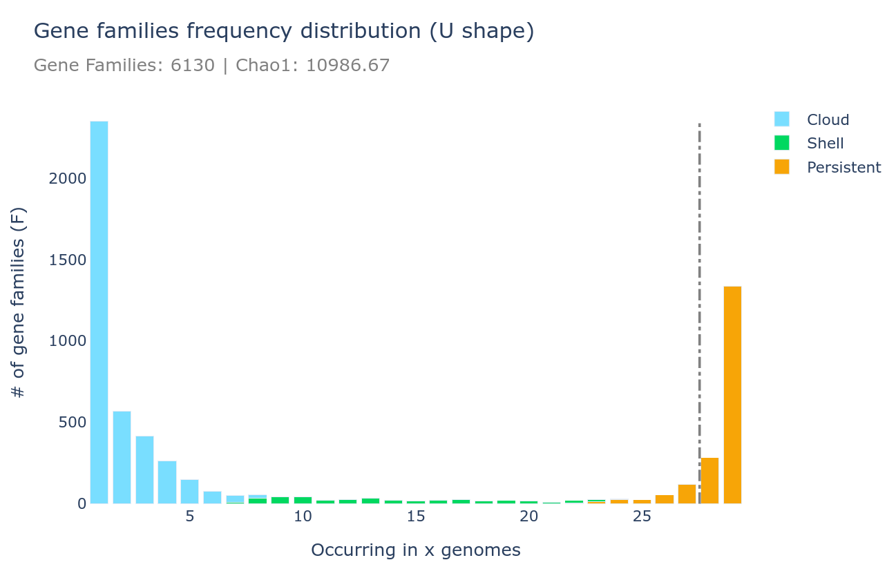
U-shape plot

A U-shaped plot is a figure showing the number of families (y-axis) per number of genomes (x-axis). The grey dashed vertical line represents the threshold used to define the soft_core. It is a .html file that can be opened with any browser and with which you can interact, zoom, move around, mouseover to see numbers in more detail, and you can save what you see as a .png image file.

It can be generated using the draw subcommand as such :

ppanggolin draw -p pangenome.h5 --ucurve

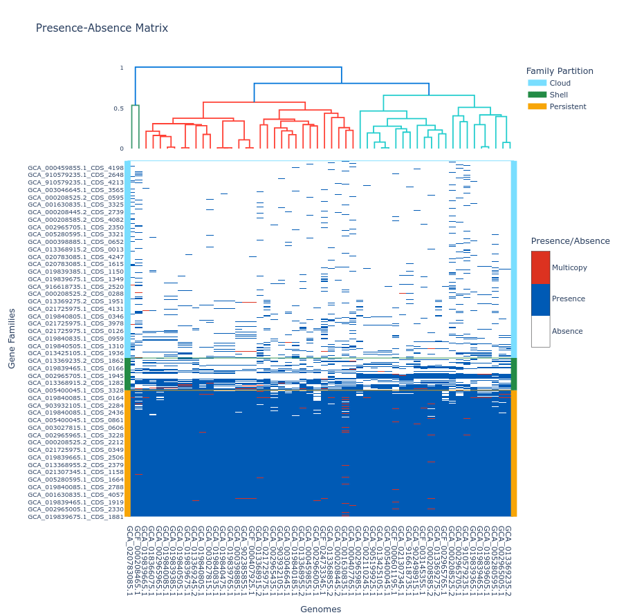
Tile plot

A tile plot is a kind of heatmap representing the gene families (y-axis) in the genomes (x-axis) making up your pangenome. The tiles on the graph will be colored if the gene family is present in a genome (either in blue or red if the gene family has multiple gene copies) and uncolored if absent. The gene families are ordered by partition and then by their number of presences (increasing order), and the genomes are ordered by a hierarchical clustering based on their shared gene families via a Jaccard distance (basically two genomes that are close together in terms of gene family composition will be close together on the figure).

This plot is quite helpful to observe potential structures in your pangenome, and can help you identify eventual outliers. You can interact with it, and mousing over a tile in the plot will indicate the gene identifier(s), the gene family and the genome corresponding to the tile. As detailed below, additional metadata can be displayed.

If you build your pangenome using a workflow subcommands (all, workflow, panrgp, panmodule) and you have more than 60k gene families, the plot will not be drawn; if you have more than 32 767 gene families, only the ‘shell’ and the ‘persistent’ partitions will be drawn, leaving out the ‘cloud’ as the figure tends to be too heavy for a browser to open it otherwise. Beyond the workflow subcommand, you can generate the plot with any number of gene families or genomes. However, no browser currently supports visualizing a tile plot containing more than 65 535 gene families or more than 65 535 genomes (for more information, refer to this Stack Overflow discussion ).

To generate a tile plot, use the ‘draw’ subcommand as follows:

ppanggolin draw -p pangenome.h5 --tile_plot

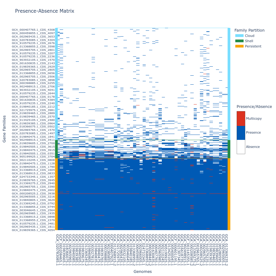
If you prefer not to include ‘cloud’ gene families, which can make the plot difficult to render in a browser, you can use the --nocloud option:

ppanggolin draw -p pangenome.h5 --tile_plot --nocloud

To include a dendrogram on top of the tile plot, use the --add_dendrogram option:

ppanggolin draw -p pangenome.h5 --tile_plot --add_dendrogram

If you have added metadata to the gene elements of your pangenome (see metadata documentation for details), you can display this metadata in the hover text by using the --add_metadata argument.

Rarefaction curve

This figure is not drawn by default in the ‘workflow’ subcommand as it requires a lot of computations. It represents the evolution of the number of gene families for each partition as you add more genomes to the pangenome. It has been used a lot in the literature as an indicator of the diversity that you are missing with your dataset on your taxonomic group (Tettelin et al., 2005). The idea is that if at some point when you keep adding genomes to your pangenome you do not add any more gene families, you might have access to your entire taxonomic group’s diversity. On the contrary, if you are still adding a lot of genes you may be still missing a lot of gene families.

There are 8 partitions represented. For each of the partitions, there are multiple representations of the observed data. You can find the observed means, medians, 1st and 3rd quartiles of the number of gene families per number of genome used. You can also find the best fitting of the data by the Heaps’ law, which is usually used to represent this evolution of the diversity in terms of gene families in each of the partitions.

It can be generated using the ‘rarefaction’ subcommand, which is dedicated to drawing this graph, as such :

ppanggolin rarefaction -p pangenome.h5

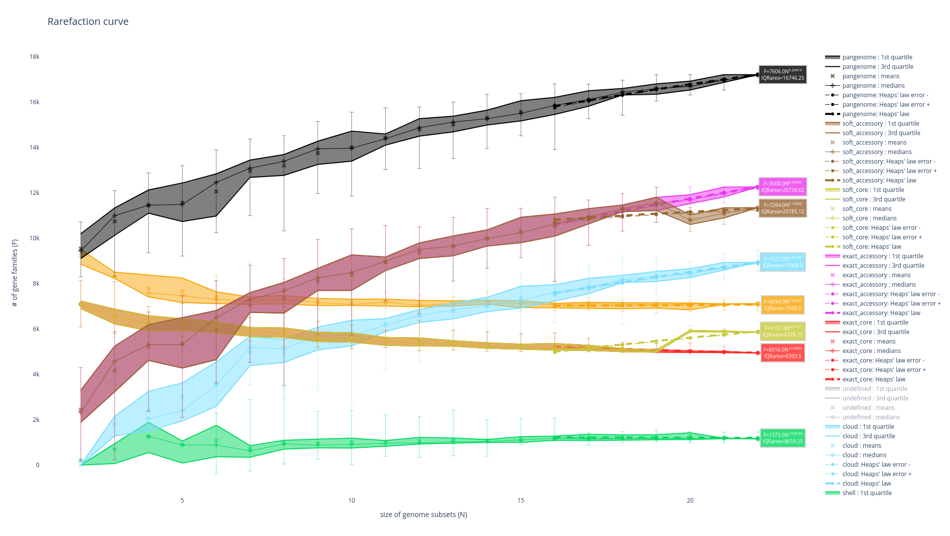
A lot of options can be used with this subcommand to tune your rarefaction curves, most of them are the same as with the partition workflow. The following 3 are related to the rarefaction alone:

• --depth defines the number of sampling for each number of genomes (default 30)

• --min defines the minimal number of genomes in a sample (default 1)

• --max defines the maximal number of genomes in a sample (default 100)

So for example the following command:

ppanggolin rarefaction -p pangenome.h5 --min 5 --max 50 --depth 30

Will draw a rarefaction curve with sample sizes between 5 and 50 (between 5 and 50 genomes will be used), and with 30 samples at each point (so 30 samples of 5 genomes, 30 samples or 6 genomes … up to 50 genomes).

Pangenome graph output

The pangneome graph can be given through the .gexf and through the _light.gexf files. The _light.gexf file will contain the gene families as nodes and the edges between gene families describing their relationship, and the .gexf file will contain the same things but also include more details about each gene and each relation between gene families. We have made two different files representing the same graph because, while the non-light file is exhaustive, it can be very heavy to manipulate and most of its content is not of interest to everyone. The _light.gexf file should be the one you use to manipulate the pangenome graph most of the time.

These files can be manipulated and visualized for example through a software called Gephi, with which we have made extensive testings, or potentially any other software or libraries able to read gexf files such as networkx or gexf-js among others. Gephi also have a web version able to open small pangenome graphs gephi-lite.

Using Gephi, the layout can be tuned as illustrated below:

We advise the Gephi “Force Atlas 2” algorithm to compute the graph layout with “Stronger Gravity: on” and “scaling: 4000” but don’t hesitate to tinker with the layout parameters.

In the _light.gexf file : The nodes will contain the number of genes belonging to the gene family, the most common gene name (if you provided annotations), the most common product name (if you provided annotations in your GFF or GBFF input files), the partitions it belongs to, its average and median size in nucleotides, and the number of genomes that have this gene family. If spots or modules are computed, it also indicates if a node belongs to them. Finally, this file also outputs the imported metadata regarding each gene family.

The edges contain the number of times they are present in the pangenome.

The .gexf non-light file will contain in addition to this all the information about genes belonging to each gene family, their names, their product string, their sizes and all the information about the neighborhood relationships of each pair of genes described through the edges.

The light gexf can be generated using the write_pangenome subcommand as such :

ppanggolin write_pangenome -p pangenome.h5 --light_gexf

while the gexf file can be generated as such :

ppanggolin write_pangenome -p pangenome.h5 --gexf

JSON

The json’s file content corresponds to the .gexf file content, but in json rather than gexf file format. It follows the ‘node-link’ format as shown in this example in javascript, or as used in the networkx python library and it should be usable with both D3js and networkx, or any other software or library that supports this format.

The json can be generated using the write_pangenome subcommand as such :

ppanggolin write_pangenome -p pangenome.h5 --json

Pangenome metrics

After computing a pangenome, it’s interesting to get some metrics about it. The aim of the metrics subcommand is to compute comprehensive metrics describing the pangenome.

All the metrics computed are saved in the pangenome file and are displayed by the info subcommand with the flag --content.

Genomic fluidity

The genomic fluidity is described as a robust metric to categorize the gene-level similarity among groups of sequenced isolates. more information here

We have added the possibility to get genomic fluidity for the whole pangenome or for a specific partition. Genomic fluidity is computable as follows:

ppanggolin metrics -p pangenome --genome_fluidity

Genomes_fluidity:
    all: 0.139
    shell: 0.527
    cloud: 0.385
    accessory: 0.62

all correspond to all the family in the pangenome (core and accessory)

Note

Currently, the metrics command only computes fluidity. However, additional metrics may be added in the future. If you have any ideas for metrics that describe the pangenome, please open an issue!

Pangenome info

The info command in PPanGGOLiN enables users to acquire comprehensive insights into the contents and construction process of a pangenome file.

Different types of information can be displayed using various parameters, such as --status, --parameters, --content, and --metadata. When no flag is specified, all available outputs are displayed.

ppanggolin info -p pangenome.h5

The info command generates information in YAML format, displaying the results directly in the standard output without writing to any files.

Overview of info --content Output

The --content option with the info command exhibits general statistical data about your pangenome:

1. General Metrics:

   • Presents a comprehensive count of genes, genomes, gene families, and edges within the pangenome graph.

2. Partitioned Metrics:

   • Provides detailed information for each partition, including gene counts and presence thresholds for persistent, shell, and cloud families among genomes.

3. Number of Partitions:

   • Indicates the total count of partitions in the pangenome.

4. Genome Fluidity:

   • If computed through the ‘metrics’ command, displays genome fluidity values across all partitions and within each partition.

5. Regions of Genomic Plasticity (RGPs):

   • Exhibits counts of Regions of Genomic Plasticity (RGPs) and spots of insertion if predicted using commands such as ‘all’, ‘panrgp’, ‘rgp’, or ‘spot’.

6. Modules:

   • Shows counts of modules and associated gene families if predicted using commands like ‘module’, ‘panmodule’, or ‘all’. Additionally, provides partition composition percentages for these modules.

Overview of info --parameters Output

This option displays the PPanGGOLiN parameters used at each analysis step. The output can be utilized as a configuration file for other PPanGGOLiN commands to replicate the same parameters. Refer here for more details on the configuration file .

Overview of info --status Output

Using this option, users can check what analysis have been conducted to obtain the pangenome file.

Overview of info --metadata Output

When metadata has been added to the pangenome elements, this option showcases which elements possess metadata and their respective sources. Find more details on metadata here.