Quick usage
PPanGGOLiN complete workflow analyses
We tried to make PPanGGOLiN relatively easy to use by making a ‘complete workflow’ subcommand called all.
It runs a pangenome analysis whose exact steps will depend on the input files you provide it with.
In the end, you will have a partitioned pangenome graph with predicted RGP, spots and modules.
The minimal subcommand only need your own annotations files (using .gff or .gbff/.gbk files)
as long as they include the genomic dna sequences, such as the ones provided by Prokka or Bakta.
ppanggolin all --anno genomes.gbff.list
It uses parameters that we found to be generally the best when working with species pangenomes.
The file genomes.gbff.list is a tab-separated file with the following organisation :
The first column contains a unique genome name
The second column the path to the associated annotation file
Each line represents a genome
An example with 50 Chlamydia trachomatis genomes can be found in the testingDataset directory.
You can also give PPanGGOLiN .fasta files, such as:
ppanggolin all --fasta genomes.fasta.list
Again you must use a tab-separated file but this time with the following organisation:
The first column contains a unique genome name
The second column the path to the associated FASTA file
Circular contig identifiers are indicated in the following columns
Each line represents a genome
Same, an example can be found in the testingDataset directory.
Tip
Downloading genomes from NCBI refseq or genbank for a species of interest can be easily accomplished using CLI tools like ncbi-genome-download or the genome updater script.
For instance to download the GTDB refseq genomes of Bradyrhizobium japonicum with genome updater, you can run the following command
genome_updater.sh -d "refseq" -o "B_japonicum_genomes" -M "gtdb" -T "s__Bradyrhizobium japonicum"
After the completion of the all command, all of your genomes have had their genes predicted, the genes have been clustered into gene families, a pangenome graph has been successfully constructed and partitioned into three distinct partitions: persistent, shell, and cloud. Additionally, RGP, spots, and modules have been detected within your pangenome.
The results of the workflow is saved in the pangenome.h5 file, which is in the HDF-5 file format. When you run an analysis using this file as input, the results of that analysis will be added to the file to supplement the data that are already stored in it. The idea behind this is that you can store and manipulate your pangenome with PPanGGOLiN by using this file only. It will keep all the information about what was done, all the parameters used, and all the pangenome’s content.
Tip
Many option are available to tune your analysis. Take a look here.
Usual pangenome outputs
The complete workflow subcommand all automatically generates some files and figures.
Here, we are going to describe several of these key outputs that are commonly used in pangenomic studies as these files illustrate the pangenome in different ways.
Statistics and metrics on the pangenome
Statistics about genomes
PPanGGOLiN generates a tab-separated file called genome_statistics.tsv describing the content of each genome used for building the pangenome.
It might be useful when working with fragmented data such as MAGs or in cases where there is a suspicion that some genomes might be chimeric or fall outside the intended taxonomic group (as those genomes will be outliers regarding the numbers in this file).
The first lines starting with a ‘#’ are indicators of parameters used when generating the numbers describing each genome, and should not be included when loading the file into a spreadsheet. However, if you load this file using R, these lines will be automatically skipped
This file is described in the documentation here.
Note
This command will also generate the ‘mean_persistent_duplication.tsv’ file.
Gene presence absence
PPanGGOLiN generates presence absence matrix of genomes and gene families called gene_presence_absence.Rtab. This format mirrors the structure of the gene_presence_absence.Rtab file obtained from the pangenome analysis software Roary.
More information about this file can be found here
mean persistent duplication
PPanGGOLiN generates a TSV file called mean_persistent_duplication.tsv. This file lists the gene families along with their duplication ratios, average presence in the pangenome, and classification as ‘single copy markers’.
More information about this file can be found here
Figures
U-shaped plot: gene families frequency distribution in pangenome
PPanGGOLiN generates a U-shaped plot called Ushaped_plot.html.
A U-shaped plot is a figure presenting the number of families (y-axis) per number of genomes (x-axis).
The file can be opened in any browser and allows for interaction, zooming, panning, and hovering over numbers for more detail.
Additionally, it is possible to save the displayed content as a .png image file.
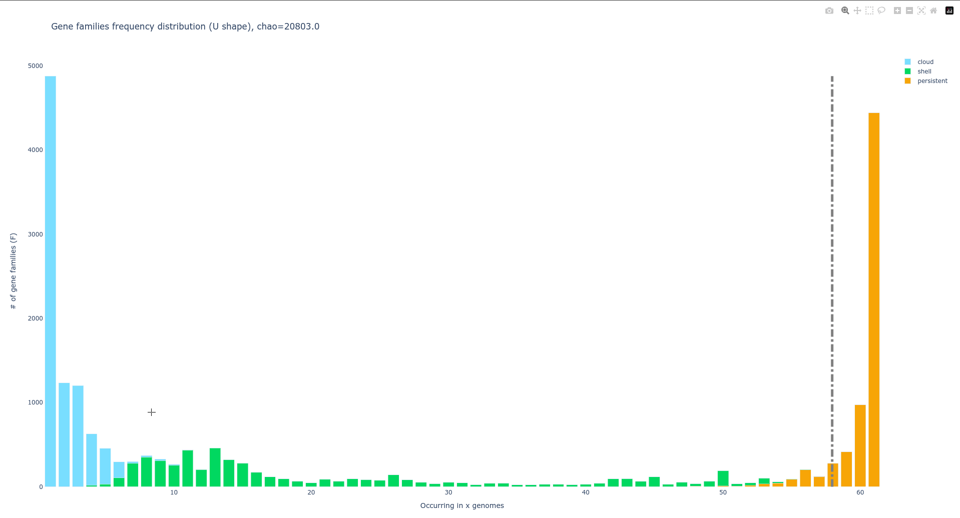
A dotted grey bar on the graph represents the soft core threshold which is the lower limit for which families are present in the majority of genomes. By default, this value is 95% (so families are in more than 95 genomes).
Additional information on this file and instructions for modifying default parameters can be found at here.
Tile plot: detect pangenome structure and outlier
A tile plot is a heatmap representing the gene families (y-axis) in the genomes (x-axis) making up your pangenome. The tiles on the graph will be colored if the gene family is present in a genome and uncolored if absent. The gene families are ordered by partition, and the genomes are ordered by a hierarchical clustering based on their shared gene families (basically two genomes that are close together in terms of gene family composition will be close together on the figure).
This plot is quite helpful to observe potential structures in your pangenome, and can also help you to identify eventual outliers. You can interact with it, and mousing over a tile in the plot will indicate to you which is the gene identifier(s), the gene family and the genome that corresponds to the tile.
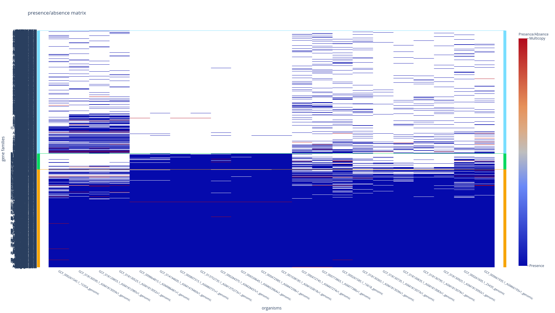
With the workflow subcommands (all, workflow, rgp and module), if you have more than 500 genomes, only the ‘shell’ and the ‘persistent’ partitions will be drawn, leaving out the ‘cloud’ as the figure tends to be too heavy for a browser to open it otherwise.Refer to here for instructions on how to add the cloud if necessary.
Rarefaction curve: an indicator of the taxonomic group diversity
The rarefaction curve represents the evolution of the number of gene families for each partition as you add more genomes to the pangenome. It has been used a lot in the literature as an indicator of the diversity that you are missing with your dataset on your taxonomic group. The idea is that if at some point when you keep adding genomes to your pangenome you do not add any more gene families, you might have access to your entire taxonomic group’s diversity. On the contrary, if you are still adding a lot of genes you may be still missing a lot of gene families.
There are 8 partitions represented. For each of the partitions, there are multiple representations of the observed data. You can find the observed: means, medians, 1st and 3rd quartiles of the number of gene families per number of genomes used. And you can find the fitting of the data by the Heaps’ law, which is usually used to represent this evolution of the diversity in terms of gene families in each of the partitions.
Note
The rarefaction curve is not drawn by default in the ‘workflow’ subcommand as it requires heavy computation.
To compute it add the option --rarefaction to any workflow subcommands (all, workflow, rgp and module) or refer to here to generate it from a pangenome file.
Pangenome graph outputs
The pangenome’s graph can be given through multiple data formats, in order to manipulate it with other software. All the formats provided by PPanGGOLiN are describe here
The pangenomeGraph_light.gexf file is a simplified version of the graph, containing gene families as nodes and edges describing their relationships. While not exhaustive, it is easier to manipulate and provides sufficient information for most users.